How To Add Conditional Formatting To Cells In Google Sheets
Google has rolled out conditional formatting for its online spreadsheet app Google Sheets. It’s a reason to rejoice because this feature isn’t about fancy or impressive looking cells. If you’ve ever used the feature of the same name on Microsoft Excel, you know it can be used to differentiate cells based on their value. The Conditional Formatting feature in Google Sheets lets you enter a differentiating criteria based on text, numerical, or date value. You can also enter a custom differentiating value. If the app identifies a cell that meets the criteria i.e. the rule(s) you applied, it will format the cell differently. What’s more is that you can apply multiple rules and choose the order they are executed in. Here’s a quick run down of the feature. It’s been released, partially on the Android version.
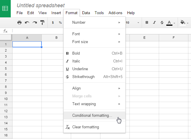
To access the Conditional Formatting dialog box go to the Format tab and select ‘Conditional Formatting’.
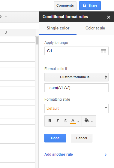
You can format cells based on the following criteria;
- Cell is empty
- Cell is not empty
- Text contains
- Text does not contain
- Text is exactly
- Date is
- Date if before
- Date is after
- Greater than
- Greater than or equal to
- Less than
- Less than or equal to
- Is equal to
- Is not equal to
- Is between
- Is not between
- Custom Formula
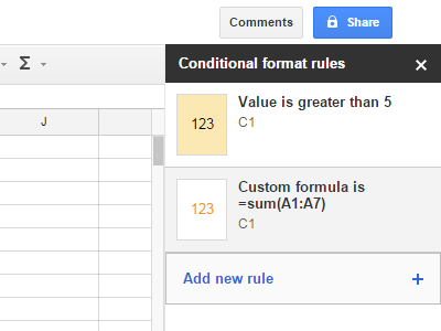
Once you click ‘Done’ you can add a second rule and then drag & drop one rule over the other to choose the order the rules are executed in.
The custom formatting option lets you define a value or formula as a differentiator. For all rules applied, you can use one of the default formatting styles of you can create your own. The feature is pretty good but sadly doesn’t have a rule for formatting cells based on date range.


