How to Use Excel SUMIF With Multiple Criteria: 3 Best Examples
Do you need to add up values of a specific column when a corresponding value in another column matches certain conditions? You need to try Excel SUMIF with multiple criteria.
Read on to learn the basics of the SUMIF formula and how to apply it in different situations.

What Is the Excel SUMIF Function?
While the SUM function just calculates the total of any cell range, SUMIF goes a step more and lets you include conditions like range and criteria. If the data fulfill the given criteria, Excel will compute the sum in the cell where the formula exists.
The formula looks like the following:
=SUMIF(range, criteria, [sum-range])
Where:
- The first input is the cell range where the target exists, like a name, value, text, etc.
- Now, you type in the criteria from the cell range. It could be a value or text.
- The final input is the corresponding cell range where the value for the target exists and needs to be added up.
Excel SUMIF With Multiple Criteria: Example #1
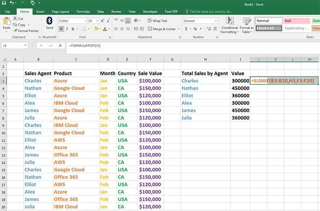
Suppose you’ve got a sales sheet showing the agent name, product, the month of sales, country, and sale value. From this data, you need to extract agent-wise sales vale across all products, months, and countries. Follow these steps:
- Go to a cell where you need the sales value.
- Copy-paste the following formula in the cell and hit Enter.
=SUMIF(B3:B20,H3,F3:F20)
The formula instructs Excel to scan through cell range B3:B20 for the value mentioned in cell H3 and compute the sum for corresponding cells in the Sale Value column, i.e., F3:F20. Instead of H3, you can use the text Charles within double-quotes.
Excel SUMIF With Multiple Criteria: Example #2
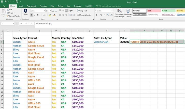
Let’s say that you need sales value for the sales agent, Alex, only for Jan. Here, you’ll need to use SUMIFS, a variation of the SUMIF formula that allows you to add up to 127 criteria. Here’s how:
- In the target cell, copy-paste the following formula and hit Enter.
=SUMIFS(F3:F20,B3:B20,B6,D3:D20,D3)
Here, the first cell range is for the values to be summed up as the Sale Value. Next, you start inserting your criteria like B3:B20 for the Sales Agent and B6 is the criteria for Alex. The other criteria are for Jan, which is D3:D20, and D3 denotes Jan.
Excel SUMIF With Multiple Criteria: Example #3
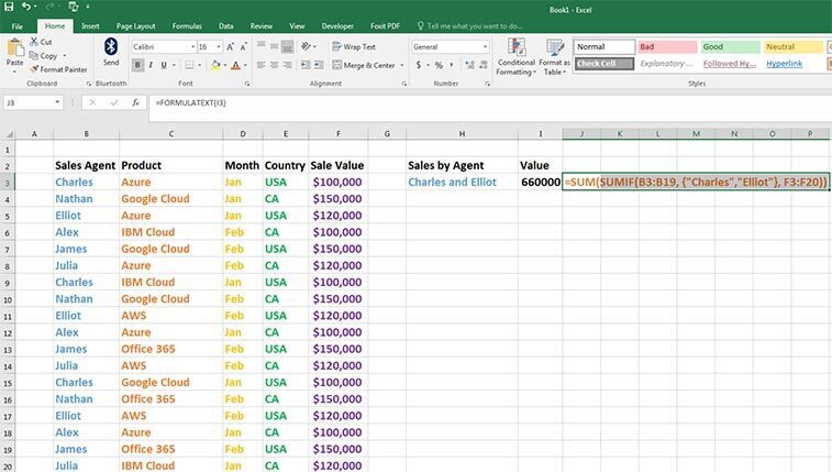
You can also simply combine the SUM and SUMIF functions to calculate Sale Value for more than one Sales Agent in a single cell. Here’s how to do it:
- Insert the following formula in any cell and hit Enter.
=SUM(SUMIF(B3:B19, {"Charles","Elliot"}, F3:F20))
The above formula is a combination of SUMIF and SUM to easily calculate total sales by multiple agents instead of using two SUMIF functions.
Conclusion
So far, you’ve learned about the SUMIF function in Excel, its syntax, arguments, etc. Moreover, you’ve also enlightened yourself with various real-life examples where you can fit Excel SUMIF with multiple criteria and get actionable insights from your Excel worksheet.
You may also be interested to know how to add developer tab in Excel.