HLOOKUP Function In Excel 2010

Excel HLOOKUP function can be used when you are dealing with huge datasheet and need to look up the values of the specific record. HLOOKUP stands for Horizontal lookup, used to find specific data from the datasheet. Unlike VLOOKUP function, it looks for the values horizontally which enables the user to extract a complete record. This post elaborates how & where you can use HLOOKUP function.

Launch Excel 2010, and open a datasheet on which you want to apply HLOOKUP function.

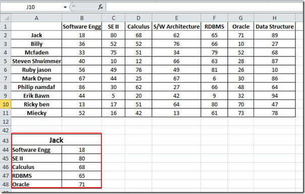
For instance, we have included student grading sheet containing courses name fields and a field containing name of the students as shown in the screenshot below.

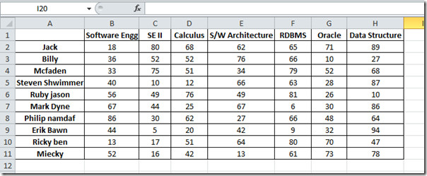
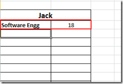
Now we want to apply HLOOKUP function, for this we will start off with adding a new row in which we will be looking up for the data of specific student. Suppose we are dealing with a gigantic datasheet containing loads of student records, in this scenario if we want to look up for the record of student Jack, then we will add the row label by the name of student and start pulling the marks he secured from each each Course column; e.g. Software Engg, Se II etc.

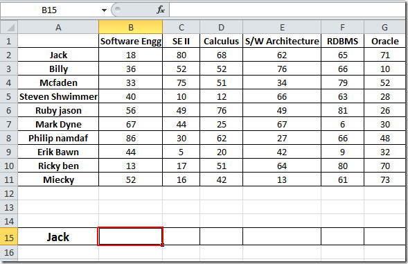
Now we will be writing formula adjacent to Jack cell, Unlike VLOOKUP function, it looks for data horizontally, The syntax of HLOOKUP function is;

=HLOOKUP(lookup_value, table_array, row_index_num, [range_lookup] )

The first parameter of the formula lookup_value defines the value of the number which we will be looking in the specified row. We need to lookup the mark in the newly created cell. The next parameter, table_array defines the table array we will be referring to in our case it will be portion of datasheet containing courses labels, with corresponding data (courses with marks secured ). row_index_num defines, which row we want to extract values to show, in our case it is the second row that contain respective course marks. [range_lookup] lets you to choose an option  either TRUE(approximately matching of values) or FALSE (Exact matching of values).

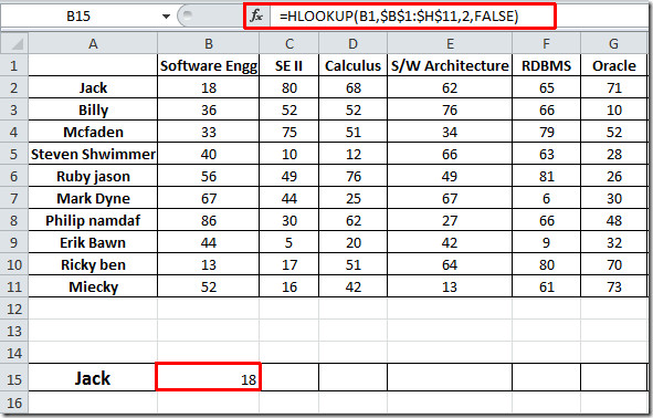
We will write this function in the cell adjacent to Jack cell, it will go like this;

=HLOOKUP(B1,$B$1:$H$11,2,FALSE)

In the formula parameters, B1 is cell of column Software Engg which contain marks secured by the student Jack, B1:H11 is the array of the data containing all courses labels and their respective values (use absolute referencing with $ sign), 2 in the formula means that values from second row will appear, and FALSE defines that we need exact match.

As you can see in the screen shot below that, the formula will yield 18 the marks secured by Jack in Software Engg course (at B1 location)

Now if you want to know marks secured by Jack in each course, just drag the plus sign across the row, as shown in the screenshot below.

There is another interesting way in which HLOOKUP function can be used, in this we will be creating exclusive table for student jack and looking up for the marks, by specifying course name, as shown in the screenshot below.

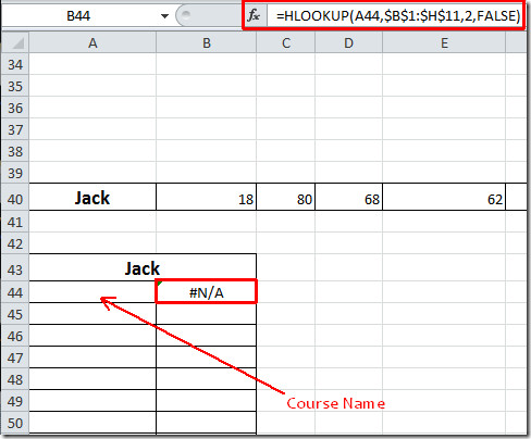
The whole formula is the same except the first parameter (A44), actually it is referring to the cell in which will write the course name. Now when we will specify course name, corresponding marks value will automatically appear.

Now apply it over the table and make an exclusive one for student Jack.

You can also check out our previously reviewed guides on VLOOKUP Function In Excel & How to embed videos in Excel 2010.

Read Full Bio

Usman Javaid

Follow me on Google+

Latest from Author

How To Create A Portable Windows 8 Enterprise To Go Workspace How To Install Windows 8 As Guest OS Using VMware Player