Guide On Excel 2010 Data Bars

Excel 2010 Data Bars makes it easier to observe that how data values relate to each other. This feature represents data graphically inside the cell, and helps user to compare data cells more effectively and efficiently by adding bars, which defines the data of the cell. It is better to represent the data graphically rather then using orthodox Conditional Formatting style. This post will cover how to make the most of Data Bars, in a simple datasheet.

Launch Excel 2010, create a new datasheet or open an existing one to apply data bars over the desired cells.

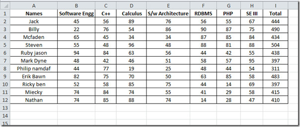
For Instance, we have student record datasheet, containing marks obtained in each course, there are 7 courses in total, so we have seven columns with their names as column headings and, a Total column which contains sum of marks obtained by each student (out of 700).

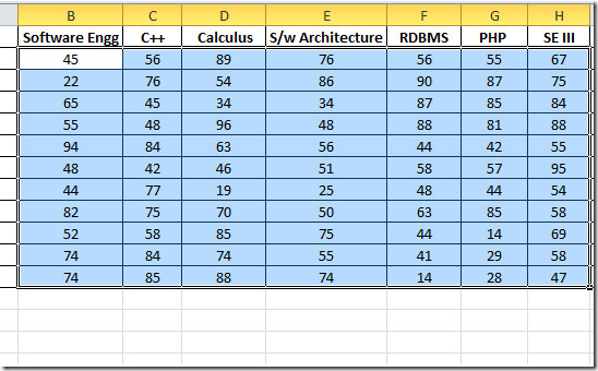
Now we want to apply Data Bar on each cell, select the portion of the data on which you want to apply it.

selected data

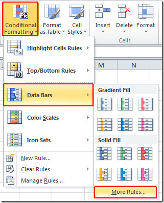
Navigate to Home tab, click Conditional Formatting, and from Data Bars menu, click more rules to customize the rules.

data bar rules 1

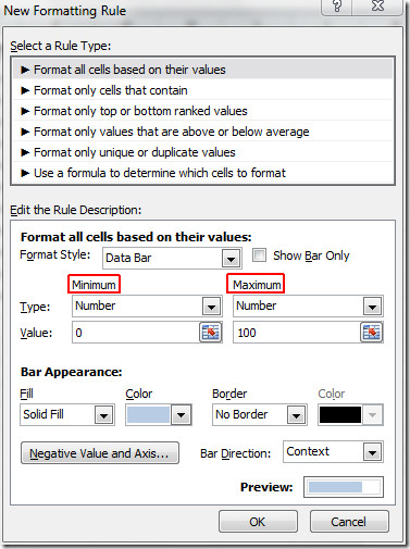
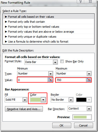
You will reach New Formatting Rule dialog. Under Select a Rule Type, select rule which best suits your data sheet. Under Rule Description, select Data Bars from Format Style, enable Show bar Only option to show only data bars without data in the cells. Under Minimum & Maximum type minimum and maximum value you want set for the selected portion of data. Under Bar Appearance you can play with different options to make your data bars more prominent by choosing color, Fill type (Solid, Gradient), Border style and color.

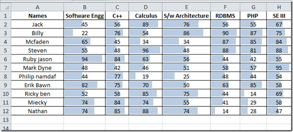
We will choose 0 and 100 as minimum and maximum values (as every course carries 100 marks, that will show data bar range in the cell, if fully filled means student secured 100 marks), and give data bars light shade of color to make data value apparent.

data bar formatting

Data Bars will be appeared as shown in the screenshot below.

data bars marks

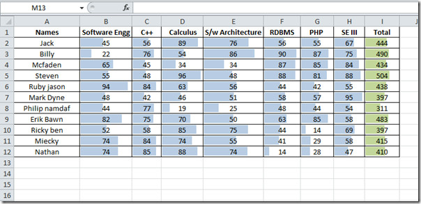
Now we want to show data bars on Total Column that carries total marks obtained by each student. Select Total column, and navigate to New Formatting Rule dialog. Now choose 0 and 700 (as there are 7 courses in total carrying 100 marks) as minimum and Maximum values respectively. Change the color of the data bar to make it distinguishable from the rest of the data cells. Click OK to continue

total column data bar 1