Excel 2010: Using SUMPRODUCT Function
Excel SUMPRODUCT is one of the most used function. Because of it’s versatility, it can be used in numerous ways. This function can handle array in a simple way, giving novices an option to use array without comprehending the structure of it. It can manipulate up to 25-30 arrays, requires list of array as argument; =SUMPRODUCT(array1, array2….). So you just need to specify range of array in your worksheet. Primarily it is used for adding and then multiply the values stored in array. This post will be putting some light on how to use this function in your spreadsheet.
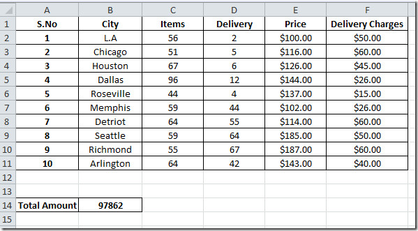
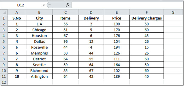
Launch Excel 2010 and open a spreadsheet on which you want to apply SUMPRODUCT function. For Instance, we have included a spreadsheet, containing records of Item & it’s respective price and number of products to be delivered, and corresponding charges as; Items, Delivery, Price, and Delivery Charges, as shown in the screenshot below.
Now we want to find out Total amount to be paid by the customers, including all the charges from every city. For evaluating total amount, old-school method can be used, but it would be hectic to write one. We will be using SUMPRODUCT function to evaluate the Total amount. We will start off with including row label Total Amount beneath the table and in it’s adjacent cell we will be writing the formula.
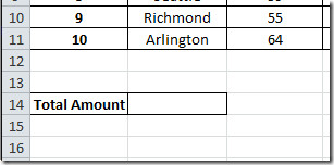
For calculating total amount we will write formula like this;
=SUMPRODUCT(C2:D11,E2:F11)
The first argument in the formula is C2:D11, this marks up the location of array1, which contains Items & Delivery field, and the second parameter E2:F11 which contains items price and delivery charges.
For example we need this sort of calculation for desired result; (56*100)+(2*100) and so on. It will evaluate by, multiplying number of items sold with it’s respective Prices and Delivery with its Delivery charges, as shown in the screenshot below.
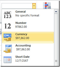
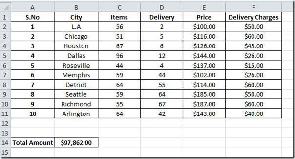
Now we will be changing the value into currency value. From Home tab, under Number group, click drop-down button, and click Currency.
You can also check out previously reviewed Excel Functions; SUMIF, COUNTIF, VLOOKUP, HLOOKUP ,PMT, and LEN.

There is a typo in the following instructions:
For example we need this sort of calculation for desired result; (56*100)+(2*100) and so on. It will evaluate by, multiplying number of items sold with it’s respective Prices and Delivery with its Delivery charges, as shown in the screenshot below. CALCULATION OF ROW 2 SHOULD READ “(56*100)+(2*50)”.
I get 100888 from your example instead of 97862.
You will get 97862 if you change the price to match what he has in the second table
For example we need this sort of calculation for desired result; (56*100)+(2*100) and so on. Should this not say (56*100)+(2*50)?
Yes
the formula does not return what he shows-Column F is used in the array but he doesn’t reference how it is used in the calculation – given his example I do not understand this function any better than I did before I saw this example – 0 stars for usefulness
A very handy use of the SUMPRODUCT fn is to return Total Taxation from a table of Marginal Tax Brackets and their associated Rates, eg:
Given Tax Threshold Marginal Tax Rate Differential Rate Tax Threshold), (Taxable Income-Tax Threshold), Differential Rate)
Note inclusion of the double minus sign.
Why we use double minus?
it’s reads it is, its is the possessive form.