Excel 2010: Select / Reselect Data Source Of Chart
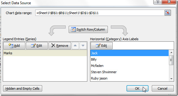
Excel 2010 provides a simple way to select the data source of charts and graphs, so that the entire table’s values can be easily plotted. However, once the chart is created, one may need to change the chart ranges by manually tweaking the values. If you want to re-select the chart source data, like you did while creating the chart, Excel 2010 offers you one click option. The Select Data option is included in the Design chart tab, which can be used after selecting the chart area. Once the tab appears on the ribbon, just click Select Data option from Data group to bring up Souce Data Source dialog to modify the data range by defining the columns and rows range. You can easily select the data source using the mouse, or manually enter the fields that you wish to include. It lets you switch row/column between original data source and imported data source, so that you can easily include the columns/rows you want to show in your chart, and remove the unnecessary ones. In addition, you can also view the hidden and empty cells and choose to show empty cells as gaps or zero on the chart.
In order to select the data source of a chart, select the chart and head over to the Design tab and click Select Data.

The Select Data Source dialog will appear. Here, you can change the data source, edit horizontal and vertical axis. Clicking the Hidden and Empty Cells button opens the Hidden and Empty Cells Settings dialog, allowing you to enable/disable show data in hidden rows and columns option, and show empty cells in the data source as gaps or zeroes. Once done, click OK, you will see the changed data source highlighted in the chart.

