Excel 2010: Matrix Inverse Function (MINVERSE)
Previously we have covered how to evaluate the determinant of matrix. Now we will be focusing on how to find out inverse of the matrix which mainly requires multiplication of determinant with matrix ad-joint. The old-school method for evaluating inverse is very tedious but with Excel MINVERSE function, we can evaluate it instantly. We just need to write or specify data range values in matrix as argument of the function.
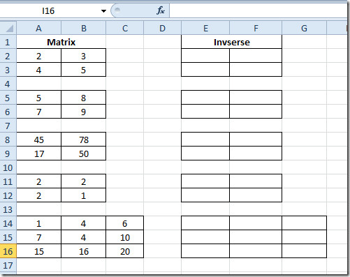
Launch Excel 2010 spreadsheet containing data in matrices. For instance, we have included spreadsheet containing fields; Matrix and Inverse.

As you have noticed that there are three 2×2 matrices and one 3×3 matrix, we will be finding out inverse of the matrices through Excel inherent function rather than applying old-school method for evaluating matrix inverse which is;
Inverse (A)= |A| Matrix (Adj [A])
You must have been familiar with the evaluation process, it becomes so complex and tedious to manage. But we will be using MINVERSE function which will yield inverse of matrix instantly.
The basic syntax of the function is;
=MINVERSE(array)
Where array could be the data range or values entered in the form of array. We will be writing formula in the first matrix in Inverse column.
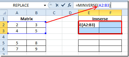
=MINVERSE(A2:B3)
Where A2:B3 is the range of matrix data in Matrix field. Select the first matrix in Inverse field i.e E2:F3. and write a formula as mentioned above.

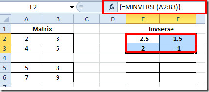
Now press Ctrl+Shift+Enter on keyboard to let Excel know that we are dealing with array. It will enclosed formula in parenthesis { =MINVERSE(A2:B3) }, as shown in the screenshot below.

Apply the formula by copying it and pasting it in other cells after selecting cells contain in other matrix.
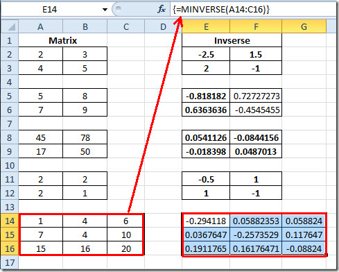
For 3×3 matrix we will again write down the formula, select the cells contain in matrix and formula will go like this;
{ =MINVERSE(A14:C16) }
It yields the result of matrix inverse in selected cells, as shown in the screenshot below.

You can also check out previously reviewed Matrix operation Function Evaluating Matrix Determinant (MDETERM) and other functions; DOLLAR, SUMPRODUCT, SUMIF, COUNTIF, VLOOKUP, HLOOKUP ,PMT, and LEN.

I see four 2×2 matrices.
Thank you
OK explanation until this point:
“Apply the formula by copying it and pasting it in other cells after selecting cells contain in other matrix.”
That part is not clear or doesn’t work.
Before typing the formula, you should select all the cells of the new inverted matrix.
And I agree it’s not clear.
How to do this with matrices of complex numbers?