How to Change Data Source and Range in Pivot Table
Pivot tables in Excel are a powerful and versatile tool for analyzing and summarizing large datasets. They enable users to organize and filter data quickly and easily, providing valuable insights and useful statistics. You can transform complex data into meaningful statistics using this tool. But what if you want to change the source and range in a pivot table in Excel? Continue reading to find out.

Changing the data source and range in a pivot table in Microsoft Excel is pretty easy. Since spreadsheets are commonly updated with new data, you will need to update your pivot table to acquire correct, fresh statistics.
There are two common scenarios for an updated dataset: Either you will have new rows (or columns) of data added to your dataset, or you will have the updated dataset in a whole new spreadsheet. In order to update your pivot table, you should change the data range in the former scenario and change the data source in the latter.
Change Data Range in Pivot Table
Let’s consider this: You have numerous new entries added to your already existing dataset, and now need to change the data range in pivot table. Here’s how to do this:
1. Open your updated Excel spreadsheet.
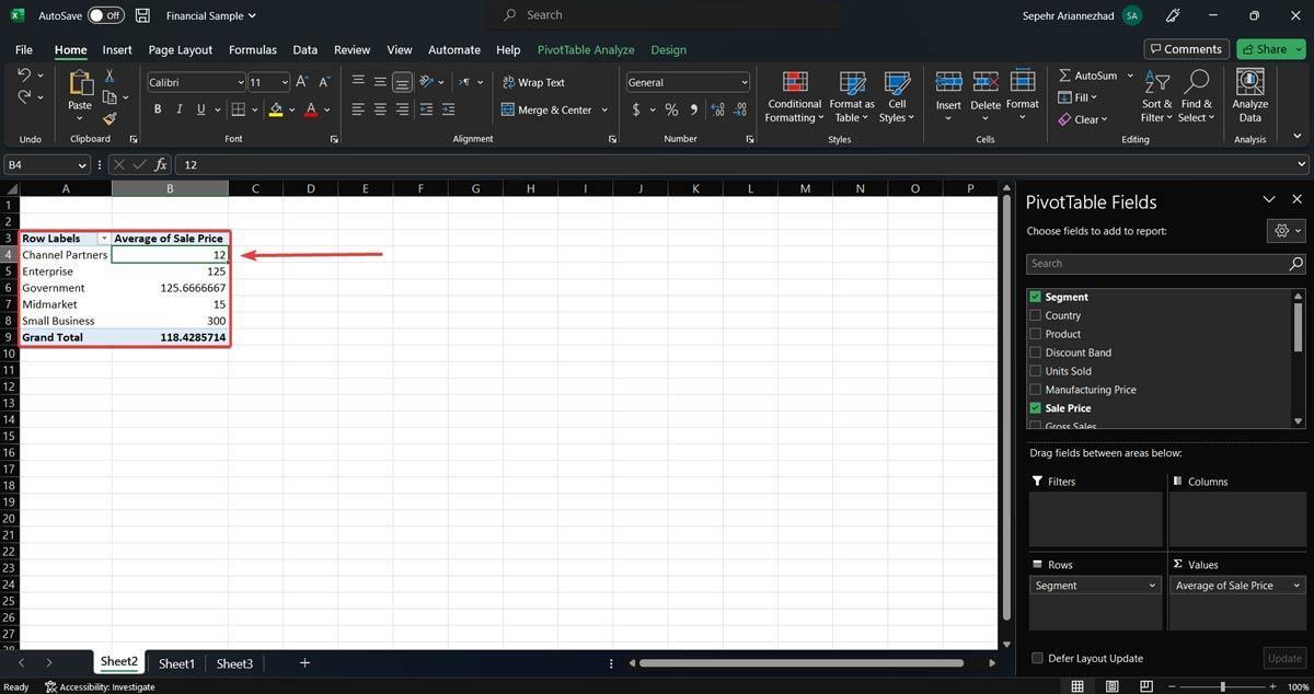
2. Select any cell located in the pivot table.
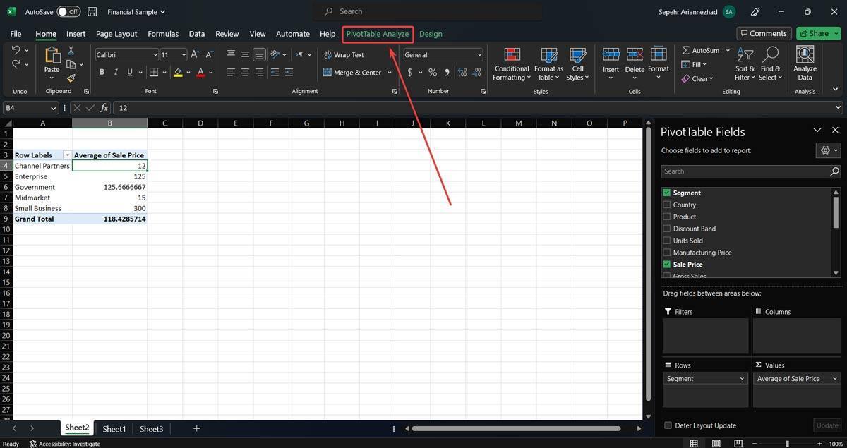
3. Select PivotTable Analyze tab from the top menu.
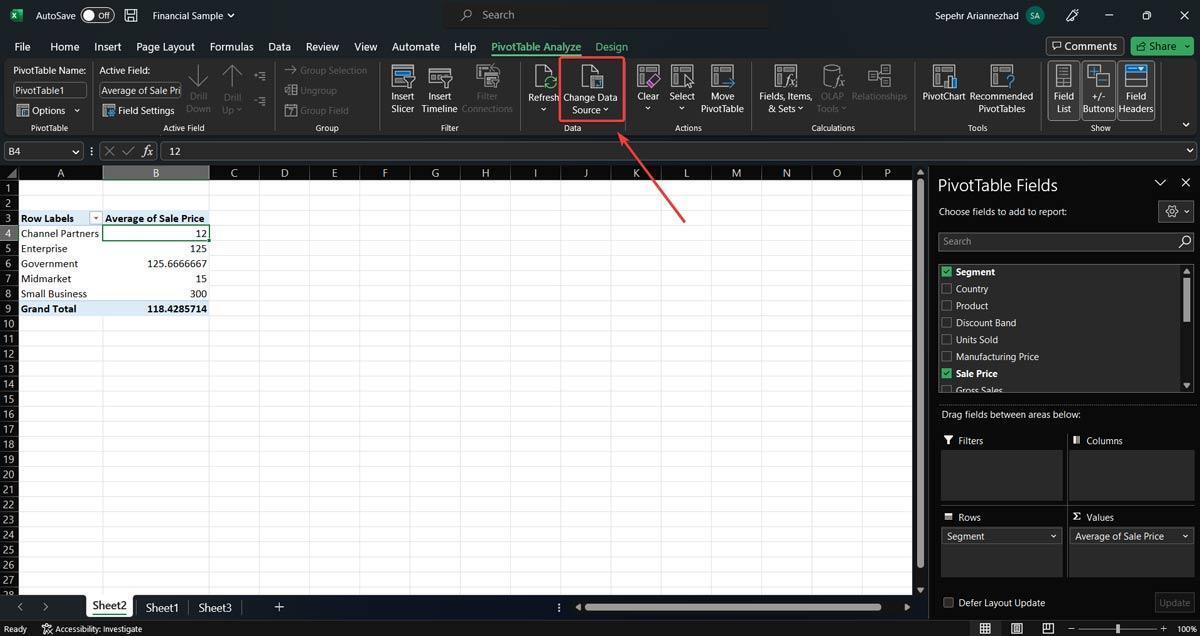
4. Select the Change Data Source option.
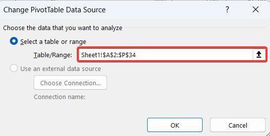
5. Select the range or table you want to analyze by either typing in the box next to Table/Range, or by selecting the range of cells with your mouse.
The format for Table/Range would be like this:
[Sheet Name]!$[Starting Column]$[Starting Row]:$[Ending Column]$[Ending Row]
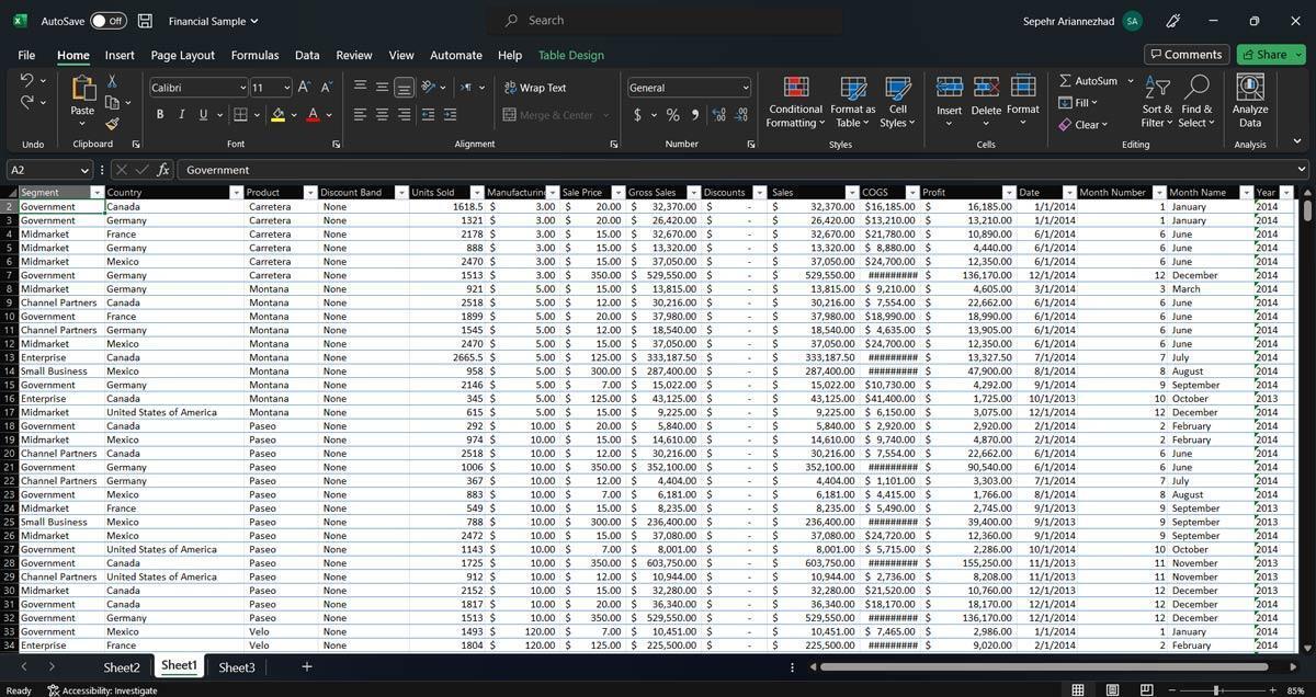
For example, the following text would select the data in cells ranging from A2 to P34 from Sheet1:
Sheet1!$A$2:$P$34
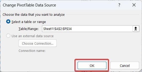
6. Select OK. Your pivot table’s range is now changed.
/
Change Data Source of Pivot Table
Now what if your new dataset is in a new worksheet? This is also easy. You just have to change the pivot table data source. Follow these steps:
1. Head over to your updated Excel spreadsheet.
2. Click on anywhere on the pivot table.
3. Click on the PivotTable Analyze tab from the top bar.
4. Click on the Change Data Source option from this tab.
5. When the Move PivotTable window is opened, go to the sheet where the new data set is by clicking on the sheet name at the bottom of the Excel window.
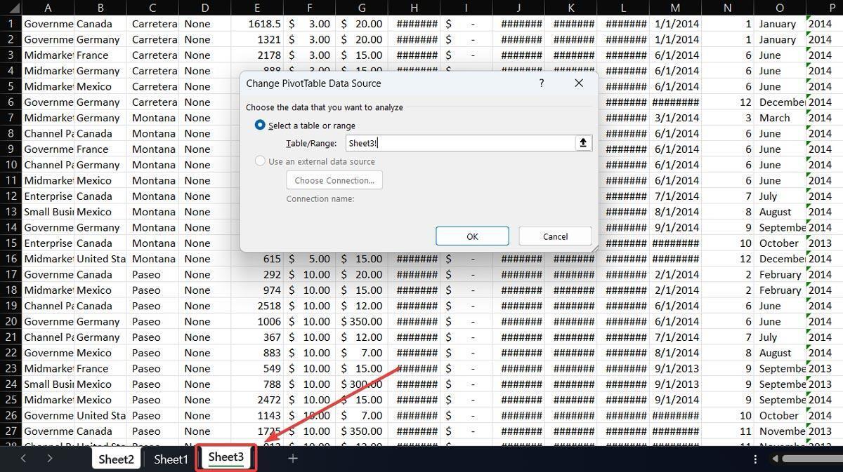
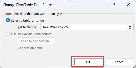
6. Select the dataset you wish to analyze by selecting the range of the dataset cells with your mouse, or by typing in the range in the Table/Range box.
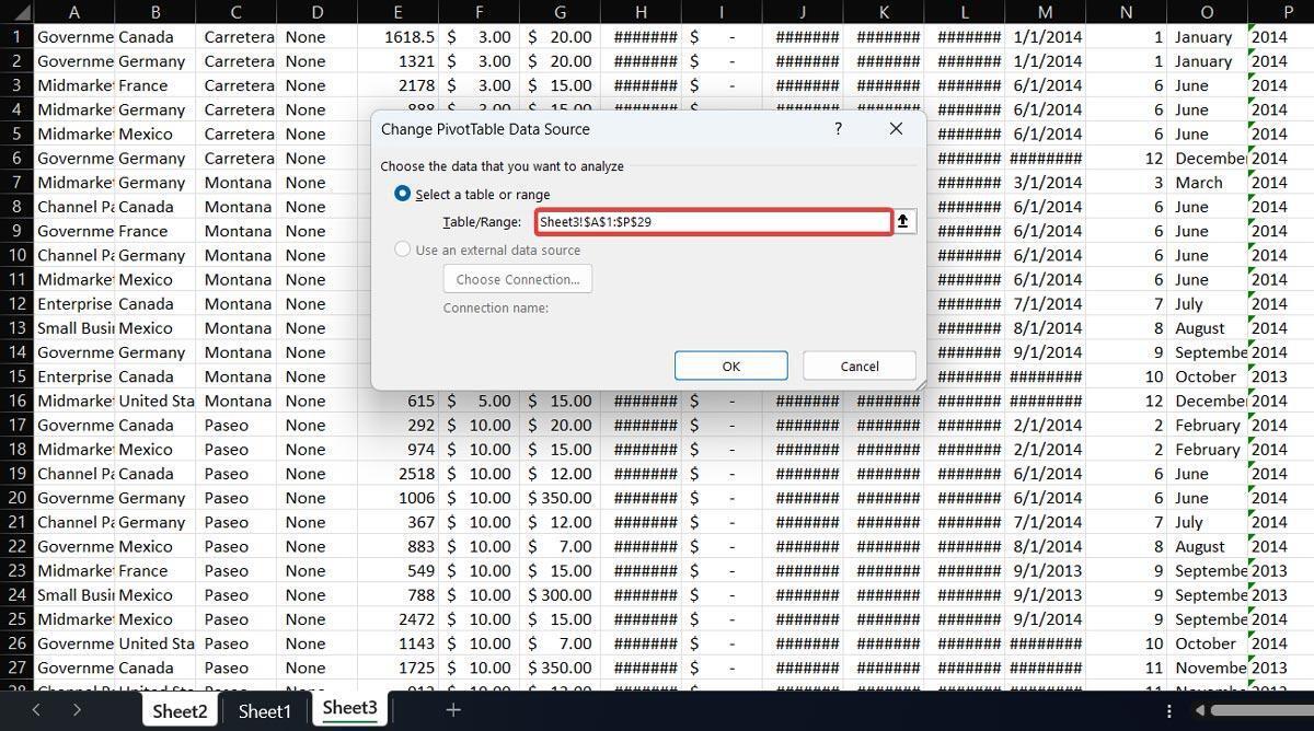
Here’s the input format:
[Sheet Name]!$[Starting Column]$[Starting Row]:$[Ending Column]$[Ending Row]
For example, selecting the data in cells A1 to P29 from Sheet3 would be by typing this into the Table/Range box:
Sheet3!$A$1:$P$29
7. Click on OK. Your pivot table is now updated.
Quick tip: As a part of Microsoft Office, Excel provides many shortcuts for different functions. For our purpose in this article, you can also select the pivot table, and then use this keyboard shortcut to directly jump into the Move PivotTable window:
Alt → J → T → I → D