Insert Slicer In Pivot Tables & Charts – Excel 2010
Excel allows user to filter data in numerous ways. Using Slicers, you will be able to depict the datasheet fields more comprehensively. This feature lets you to slice your data by showing only the element stored in the tables. However, the real usage of Slicers can be seen with pivot table. Unlike Pivot table, which pivots down the datasheet, it enables you to compare and evaluate the data from different perspectives. This post will explain how you can use Slicer with Pivot Table and Charts.
To begin with, launch Excel 2010, and open a datasheet, containing Pivot Table.
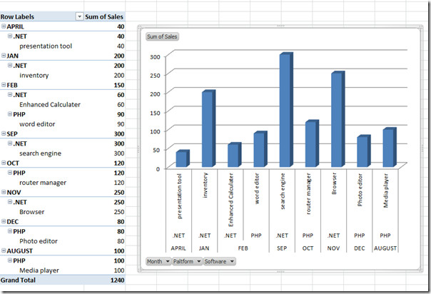
We have made Pivot Table and Pivot Chart using the above datasheet.
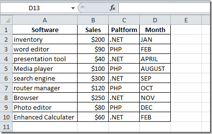
The datasheet, containing fields; Software, Sales, Platform, and Month. Datasheet shows the software developed using two platforms (PHP, .NET), its price and month in which development completed.
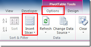
Now we want to create slicers for each category present in Pivot table. For this, select the whole Pivot table, and navigate to Options tab, click Insert Slicer.
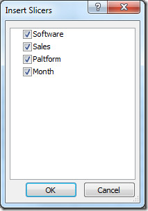
Upon click, Insert Slicers dialog will appear, containing fields of the Pivot table. Select the desired one from the list to view respective Pivot table and chart, and click OK.
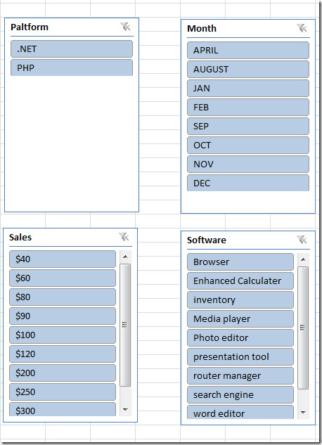
You will see box of each field, containing data as shown in the screen shot below.
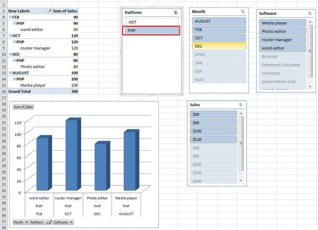
Now we want to view the software developed on PHP platform. For this, we will click PHP in Platform field box. You will see the pivot table and chart will automatically show all the info related to PHP platform, i.e, in which month it was used, which software developed on this platform and price of the software.
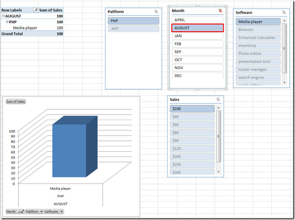
Now if we select August from Month field, then it will show all the info related with month of August, i.e, which platform was used to make which software, and what was its price.
By using Slicers you can filter down your data in more detail. Its real usage can be seen when you are dealing with huge data sheet.
You can also check out previously reviewed guides on How to make Pivot Tables & Charts and Using Camera tool in Excel.

If slicer is greyed out, you are probably running Excel in compatibility mode.
I used a slicer on a pie chart and noticed that it can only display a single slicer item. If I select multiple items, all I see on the pie chart is the first item from the selection. Has anyone else experienced that problem?
I am sorry this is my 3rd thread in an hour. I found the solution for my problem. I am not sure if you have the same issue, but its worth a try. For some reason my file was in different version format, So what you need to do is save or convert your workbook to the current version and that should highlight your slicer. Try it out and let me know.
Good luck
Aammini
This tip was very useful as I struggled for 2 days and then found it silly. I was simple save in current format. It works!!!
Thanks!!!! Very helpful
Thanks!!!! Very helpful
In fact the whole sort/filter section is grayed out. Any tip will be highly regarded.
Thanks
This is all good, however the “Insert Slicer” icon is greyed out on my toolbar even though my pivot table is active. Can you advise?
Slicer icon is grayed out in my toolbar too. I wish someone will respond to this thread.
Thanks
Make sure you click in the pivot table before you insert the slicer.